This article will describe how to use Optaplanner for job shop scheduling, using automated Caipirinha manufacturing as an example.

(By Christian „VisualBeo“ Horvat [CC BY-SA 2.0 de (https://creativecommons.org/licenses/by-sa/2.0/de/deed.en)], from Wikimedia Commons)

Introduction

The Problem

Let’s assume you are running a high volume, fully automated Caipirinha bar. Making Caipirinha involves the following processes:

• ICE: Making ice blocks from water
• POLISH: Polishing the glass
• CRUSH: Crushing some ice blocks for one glass
• CUT: Cutting lemon
• MIX: Putting crushed ice in the glass, together with all other required ingredients
• DECORATE: Decorating the glass
• CLEAN: Cleaning the glass once it has returned from the customer

Each of these processes has a specific base duration.

In your automated Caipirinha bar, you can utilize a fixed number of equipments / machines. Each machine

• is capable of running one or multiple processes (but only one at a time)
• might have an advantage or disadvantage in its processing speed, compared to other machines capable of running the same process
• takes a specific amount of idle time to be set up to execute a different process (e.g. before the ice crushing machine can do lemon cutting, it needs to get a different part mounted)

Your customers are streaming into your bar at a fairly predictable rate, but with different levels of priority. Regular customers will be served with critical priority, returning customers with major, and first time customers with minor priority. (Let’s not debate that approach here 🙂  )

Constraints

There are – in this basic example – the following constraints that MUST be met by a solution (= Hard Constraints):

• A job can only run on a machine that supports the setup required by the job type.
• Only one job can be processed at a time on a given machine

Violating hard constraints renders the solution invalid.

In addition, there are constraints that CAN be met by a solution (= Soft Constraints). This is where your optimization potential is coming from: the fewer soft constraints are violated, the better the solution:

• Search for the smallest end time across all equipments
• Do not perform / minimize the number of setup changes on machines
• Do prioritize in this sequence: critical, major, minor

Objectives

You want your Caiprinha manufacturing to work as efficient as possible, which leads us to the following objectives:

• Minimize the makespan (the total time it takes to finish all process jobs)
• Process all jobs according to their priority
• Minimize machine idle time

Task: assign all process jobs to equipments, in sequences that best meet your objectives.

What’s the deal?

In our example, we are dealing with a lot of „variables“: number of equipments, equipment capabilities, different equipment speed, number of jobs to process, different job priorities, necessity to change equipment setup (because manufacturing capacity is limited and you might have more processes than equipments), …

Taking all this into account, you are dealing with a significant problem of combinatorics (number of potential solutions), where you’d have to evaluate all these possible solutions against multiple objectives.

See Job Shop Scheduling for more information.

Job Shop Scheduling with Optaplanner

Optaplanner

Optaplanner is a free and open source constraint satisfaction solver. It allows for modeling and solving problems as outlined above, but can be applied to a variety of optimization problems, such as employee rostering, vehicle routing, …

Having worked with CPLEX solver from IBM before, there are a few points I would like to point out that I was positively surprised with when looking into Optaplanner:

• With Optaplanner, there is no need to translate from your business object model (equipments, processes, …) to a rather abstract set of data structures – if you have an application with a well defined object model, chances are good you can directly use these objects for solving optimization problems.
• Optaplanner has a more intuitive (you can have your own opinion about this) way of describing constraints and how constraint violations are treated, using a rules engine.
• The examples shipped with Optaplanner include user interfaces that allow you to follow the progress of the solving process in real time, as intuitive visualization (e.g. Gantt chart).
• Documentation is excellent, examples for a variety of problems are available. Great!

On the downside, there are a few points that I would also like to mention:

• Solving optimization problems is a CPU intense operation. Spreading solver processes across multiple cores requires some extra work in Optaplanner, and might have an impact on the quality of the end results.
• Performance is not as good as the commercial solver I mentioned, but should be good enough for many problems.

Setting up an application that embeds Optaplanner

Optaplanner can easily be embedded into any Java application. In addition, there is an Execution Server that can solve optimization problems on a remote system, based on requests (e.g. through messaging or http requests).

We will use the embedded approach for this example. Setting up a project and getting started with Optaplanner is described really well in the Optaplanner documentation, so we are skipping the details here.

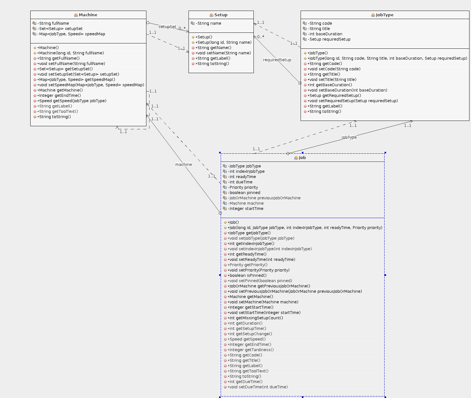
The Caipirinha manufacturing Object Model

Here are the main objects and their attributes:

Setup

• a specific machine / equipment configuration required to execute a manufacturing process
• identified by a name

Job Type

• a specific type of process
• requires exactly ONE setup
• identified by a name and code
• has a base duration

Job

• a specific task (= instance of a job type) to be processed
• is ready at a given time (cannot be started before this time)
• has a specific priority

As part of a solution, a job is assigned to a machine at a given start time. The end time is calculated based on the speed of the machine and whether or not a setup change is required for this machine in order to process this job.

Machine

• equipment or machine required to execute a job with a specific setup
• identified by a name
• can be set up / configured in 1..n ways (= supports different setups)
• can only have one specific setup at a time
• can have process times advantages (= job type runs quicker on this machine) or disadvantages (= job type runs slower on this machine)
• can only process one job at a time

Constraints Implementation

In very simple terms, Optaplanner calculates a score for each potential solution. For our use case, we will use a Hard-Soft-Score, which is a compound scoring for hard and soft constraints. Optaplanner will try to maximize the scores. A hard score lower than 0 will indicate that there is no solution to the problem. The higher the soft score, the more „optimal“ the solution.

Although there are multiple ways to implement such score calculation, we will focus on the „Drools“-based approach because it provides best performance by means of iterative score calculation. This basically means using a set of rules that are called upon changes to a solution. Rules are defined in a separate rules configuration. These rules are then supposed to add to the hard or soft score. This is where you would also implement a priority / weight of your soft constraints: some are more important than others. Identifying and using proper weights is a major task when working with optimization.

Let us review the constraints we defined, and look at how this can be implemented in our Optaplanner application:

Hard constraints:

• A job can only run on a machine that supports the setup required by the job type: Implemented in the rules configuration:

rule "Setup requirements"
    when
        Job(machine != null, missingSetupCount > 0, $missingSetupCount : missingSetupCount)
    then
        scoreHolder.addHardConstraintMatch(kcontext, - $missingSetupCount);
end

Rule „setup requirements“ is called for each job that is assigned to a machine (machine != null), initializes a variable $missingSetupCount from the missingSetupCount attribute of the job (our business object checks for missing setups), and subtracts the value from the hard score.

• Only one job can be processed at a time on a given machine

This is not explicitly modeled in our rules configuration, but enforced by the start time calculation within our Job class: if there is a previous job, the start time of the job is the end time of this previous job. This way, there can not be any overlaps.

Soft constraints:

• Search for the smallest end time across all equipments

rule "Minimize Cmax"
    when
        Job(machine != null, nextJob == null, $endTime : endTime)
    then
        scoreHolder.addSoftConstraintMatch(kcontext, - 2 * ($endTime * $endTime));
end

For jobs that are assigned to a machine AND that have no next job, add a soft score based on their end time.

• Do not perform / minimize the number of setup changes on machines

I have implemented this in two different ways: (1) have the job calculate its duration and factor in setup times, in case there needs to be a setup and (2) explicitly put a penalty on setup changes. Option 1 is implemented in our object model directly, whereis option 2 is implemented as a rule:

rule "Minimize setups"
    when
        Job(nextJob != null, setupChange == 1)
    then
        scoreHolder.addSoftConstraintMatch(kcontext, - 750000);
end

Be cautious with absolute numbers – you need to have a fairly good understand of your soft scoring range, to make sure that constraint violations are reflected to the extent you desire (weighting).

• Do prioritize in this sequence: critical, major, minor

There are three different rules for each priority level. As an example this is what one of them could look like:

rule "Critical priority"
    when
        Job(machine != null, priority == Priority.CRITICAL, $endTime : endTime, $dueTime : dueTime)
    then
        scoreHolder.addSoftConstraintMatch(kcontext, - (int)(0.8 * (($endTime - $dueTime) * ($endTime - $dueTime))));
end

For major and minor priority, lower the weight of 0.8 to e.g. 0.6 and 0.4.

For now, ignore the use of dueTime, we will get to this later. Just using the squared $endTime will do for now.

Solver configuration

To tell Optaplanner how to solve the problem, you need to provide configuration values for your specific problem as well as technical parameters (e.g. solver runtimes). Let’s look at an example:

<?xml version="1.0" encoding="UTF-8"?>
 <solver>
 <solutionClass>com.jdimension.jobshopscheduling.domain.JobAssigningSolution</solutionClass>
 <entityClass>com.jdimension.jobshopscheduling.jobassigning.domain.JobOrMachine</entityClass>
 <entityClass>com.jdimension.jobshopscheduling.jobassigning.domain.Job</entityClass>

<scoreDirectorFactory>
 <scoreDrl>com/jdimension/jobshopscheduling/solver/jobAssigningScoreRules.drl</scoreDrl>
 </scoreDirectorFactory>

<termination>
 <unimprovedSecondsSpentLimit>25</unimprovedSecondsSpentLimit>
 <secondsSpentLimit>120</secondsSpentLimit>
 </termination>
 </solver>

The solutionClass will represent a solution – jobs being assigned to machines in a specific sequence. entityClass is the „flexibility“ or planning entity in our problem. By intelligently „trying“ out changes to the planning entities and calculating hard/soft score, the solver will ultimately find a (near) optimal solution.

The second part of the configuration indicates the path to the rules configuration.

The termination part indicates „please calculate for a maximum of 2 minutes, or until you have not found a better solution for more than 25 seconds“.

Solving the problem

Solve and evaluate

To evaluate solution, you would

(1) Run the application, and evaluate the output

Is the result valid? Can you explain why a specific sequence is proposed?

(2) Fine-tune weights

Once the schedule looks valid, check and fine-tune weights of your soft constraints.

• Makespan might be sub-optimal because you put too much weight on setup reduction – causing an unbalanced result (load balancing across equipments not ideal)
• Priorities are not respected well enough: tune your weights for the job priority related rules. Determine their impact in comparison with the makespan weight. Do you have to normalize values?

The low priority customer issue

For our case, solving the problem looks valid for a given point in time.

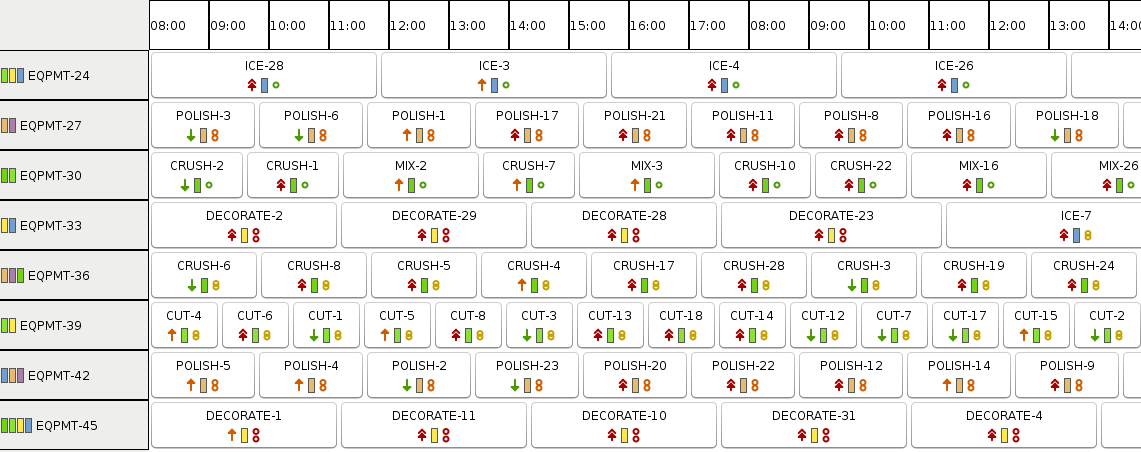
On our left we see equipments and color codes indicating their capabilities (possible setups). Our jobs setup requirements (color) all match the setups of the equipments.

We see „streams“ of equal setups (= minimize idle time), and we see high priority lots typically manufactured before lower priority lots (left icon the job).

We see a larger variation of best using equipment speed (right side icon on the jobs).

Many of the low priority jobs (first time Caipirinha bar customers) are moved to the end of the schedule. While this might make sense for a given point in time, we will run into issues with a continuous stream of new incoming jobs, which is the case for our automated Caipirinha manufacturing. With many new jobs having critical and major priority, we end up pushing out all the low priority jobs. First time customers will hardly get any Caipirinha at all! This will hurt our business, so let’s make sure that we just keep them waiting for a little (to serve our more important customers), but not starve them.

There are several ways to tackle this, and one of them is using

(Artificial) Due Dates

We are now going to put due dates on our jobs. They should be „far enough“ in the future to give enough flexibility to the solver. Defining a due date needs to be tailored to use case, can be e.g.

• just a value based on a constant duration (ready time + fixed duration)
• based on a backward propagation of a customer commitment date
• …

We will then put a penalty on the „lateness“ of jobs:

rule "Critical priority"
    when
        Job(machine != null, priority == Priority.CRITICAL, $endTime : endTime, $dueTime : dueTime)
    then
        scoreHolder.addSoftConstraintMatch(kcontext, - (int)(0.8 * (($endTime - $dueTime) * ($endTime - $dueTime))));
end

$endTime – $dueTime indicates the lateness for a given job. Note that the rule above is not ideal for jobs that are not late yet, because the lateness is negative in this case, but due to the squared value this fact is lost. You could solve this by adding a condition to the rule: dueTime < endTime

At some point in time, the „high lateness“ penalty of a low priority job will become larger than the „low lateness“ penalty of high priority job. In turn, long waiting low priority jobs will be processed before taking on new high priority jobs.

First time customers of the Caipirinha bar will only wait for specific amount of time, but they will be served.

Performance

In a set of 8 machines with 200 jobs, the problem reaches optimality in terms of the highest weighted soft constraint (minimize makespan) after only a few seconds. After ~60 seconds, the result looks good with regards to the remaining constraints, and keeps on finding slightly better results until it reaches the configured limit of 120 seconds.

The complexity of many manufacturing problems should be in the range of this problem or lower. This makes Optaplanner a viable solution for these problems.

Performance is certainly behind commercial solvers, but still I am positively surprised.

Thumbs up, Optaplanner!