This article will describe one (of possible many) solutions for solving the Fisher & Thompson Job Shop Scheduling Problem. I will use the FT10 data set, which consists of

• 10 machines
• 10 jobs with
• 10 steps each

Each job consists of many steps, that need to be processed in a given sequence. Each step needs to be performed on a specific machine.

The FT10 problem has been described in 1963 and was „unsolved“ (meaning there was no solution that was proven to be optimal) until 1989. It is a widely used dataset for solving job shop scheduling problems not just by means of Constraint Programming but also Petri Nets, Artificial Neural Networks and various flavours of heuristics.

Preparing the data

FT10 is available in the OR Library, which is a collection of data sets for Operations Research topics. The input looks like this:

Ops = [
[<0 29>, <1 78>, <2  9>, <3 36>, <4 49>, <5 11>, <6 62>, <7 56>, <8 44>, <9 21>]
[<0 43>, <2 90>, <4 75>, <9 11>, <3 69>, <1 28>, <6 46>, <5 46>, <7 72>, <8 30>]
[<1 91>, <0 85>, <3 39>, <2 74>, <8 90>, <5 10>, <7 12>, <6 89>, <9 45>, <4 33>]
[<1 81>, <2 95>, <0 71>, <4 99>, <6  9>, <8 52>, <7 85>, <3 98>, <9 22>, <5 43>]
[<2 14>, <0  6>, <1 22>, <5 61>, <3 26>, <4 69>, <8 21>, <7 49>, <9 72>, <6 53>]
[<2 84>, <1  2>, <5 52>, <3 95>, <8 48>, <9 72>, <0 47>, <6 65>, <4  6>, <7 25>]
[<1 46>, <0 37>, <3 61>, <2 13>, <6 32>, <5 21>, <9 32>, <8 89>, <7 30>, <4 55>]
[<2 31>, <0 86>, <1 46>, <5 74>, <4 32>, <6 88>, <8 19>, <9 48>, <7 36>, <3 79>]
[<0 76>, <1 69>, <3 76>, <5 51>, <2 85>, <9 11>, <6 40>, <7 89>, <4 26>, <8 74>]
[<1 85>, <0 13>, <2 61>, <6  7>, <8 64>, <9 76>, <5 47>, <3 52>, <4 90>, <7 45>]
];

Each line represents one job. The number pairs <x y> indicate the individual steps of the job, where a step needs to be processed on machine x, which takes y time units.

I converted this to an Optaplanner-friendly XML format. A job would then look like this:

<TaJob id="0">
<id>0</id>
<customId>00</customId>
<duration>29</duration>
<machine reference="2000"/>
</TaJob>

<TaJob id="1">
<id>1</id>
<customId>01</customId>
<duration>78</duration>
<predecessor reference="0"/>
<machine reference="2001"/>
</TaJob>

<TaJob id="2">
<id>2</id>
<customId>02</customId>
<duration>9</duration>
<predecessor reference="1"/>
<machine reference="2002"/>
</TaJob>

<TaJob id="3">
<id>3</id>
<customId>03</customId>
<duration>36</duration>
<predecessor reference="2"/>
<machine reference="2003"/>
</TaJob>

[...]

<TaJob id="9">
<id>9</id>
<customId>09</customId>
<duration>21</duration>
<lastStep>1</lastStep>
<predecessor reference="8"/>
<machine reference="2009"/>
</TaJob>

Each job has an ID, the duration taken from FT10, a reference to its predecessor to build the sequence of steps, and a reference to the machine it needs to run on.

I also added a „last step“ attribute so I can later easily identify the jobs that have no successor. This will help writing hard and soft constraint rules later on.

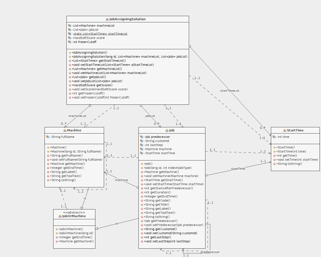
The Object Model

Our model will consist of

• Machine: required resource to process jobs (for the rest of this article, I will use „job“ for the actual step in the problem description – that is because we do not need to model jobs specifically – it is implicitly modeled through our references to a predecessor)
• Job: has an ID (generated), a predecessor job (from FT10), a reference to a machine it needs to run on (from FT10), a duration (from FT10), a „last step“ flag (generated, see above), a start time (our planning variable), an end time (calculated based on start time and duration) and a custom ID. The custom ID is generated and will help analyzing / understanding the solution. It is basically a two-digit number with job index and step index. Job 2 would contain of steps with custom IDs 20, 21, 22, 23, 24, 25, 26, 27, 28 and 29.
• StartTime: our planning variable. By changing the start time of a job, we generate different solutions.
• JobAssigningSolution: solution helper class

Objective and Constraints

Objective

Schedule all 10 jobs (100 steps) onto the 10 machines, and minimize the Makespan (time it takes to process all jobs).

Constraints

Hard Constraints

All Hard Constraints need to be satisfied, otherwise the solution is invalid.

• No overlapping jobs: a machine can only process one job at a time

I created a rule like this:look for two jobs running on the same machine, calculate their overlap and in case of overlap add a penalty to the hard score.

rule "Only one job at a time on a machine"
 when
 $leftJob : Job(machine != null, $leftId : id, $machine : machine)
 $rightJob : Job(machine == $machine, Job.overlap($leftJob) > 0, id > $leftId)
 then
 scoreHolder.addHardConstraintMatch(kcontext, - 1 * 1);
end

• Sequence requirement: a job must not start before its predecessor has finished

The rule checks all jobs that have a predecessor, calculates an integer (0/1) that indicates whether the constraint is satisfied and adds a penalty to the hard score if applicable.

rule "Sequence requirements - start after predecessor has finished"
 when
 Job(predecessor != null, $startsAfterPredecessor : startsAfterPredecessor)
 then
 scoreHolder.addHardConstraintMatch(kcontext, - $startsAfterPredecessor);
end

Soft Constraints

Soft constraints do not impact feasibility but the quality of the solution.

• Minimize the makespan (total time it takes to process all steps)

The rule applies to all jobs that are assigned to a machine and that have no successor (=last step in the job sequence). It adds a penalty to the soft score (quadratic end time).

rule "Minimize Cmax (last jobs)"
 when
 Job(machine != null, lastStep == 1, $endTime : endTime)
 then
 scoreHolder.addSoftConstraintMatch(kcontext, - 1 * ($endTime * $endTime));
end

Solver Configuration

The configuration below does the following:

• specify solution and entity (planning entity) classes
• specify the rules files implementing hard and soft constraints
• terminate the solver after a maximum of 120 seconds or after 25 seconds with no further improvements to the solution
• Use a construction heuristic for a quick identification of a first valid result

<?xml version="1.0" encoding="UTF-8"?>
 <solver>
 <solutionClass>com.jdimension.jobshopscheduling.jobassigning.domain.JobAssigningSolution</solutionClass>
 <entityClass>com.jdimension.jobshopscheduling.jobassigning.domain.Job</entityClass>

<scoreDirectorFactory>
 <scoreDrl>com/jdimension/jobshopscheduling/jobassigning/solver/jobAssigningScoreRules.drl</scoreDrl>
 <initializingScoreTrend>ONLY_DOWN</initializingScoreTrend>
 </scoreDirectorFactory>

<!-- enable this to quickly find issues with the model -->
 <!-- environmentMode>FAST_ASSERT</environmentMode -->

<termination>
 <unimprovedSecondsSpentLimit>25</unimprovedSecondsSpentLimit>
 <secondsSpentLimit>120</secondsSpentLimit>
 </termination>

<constructionHeuristic>
 <constructionHeuristicType>FIRST_FIT_DECREASING</constructionHeuristicType>
 <forager>
 <pickEarlyType>NEVER</pickEarlyType>
 </forager>
 </constructionHeuristic>

<localSearch>
 <localSearchType>LATE_ACCEPTANCE</localSearchType>
 </localSearch>
 </solver>

Boilerplate code

Based on Optaplanner examples, I created a basic Swing UI that provide color coding for all steps of a job, so one could easily identify the sequence in a larger schedule. Also, the individual assignments show the custom ID I have defined (and described earlier in this article).

Results

Running our solver yields the following result:

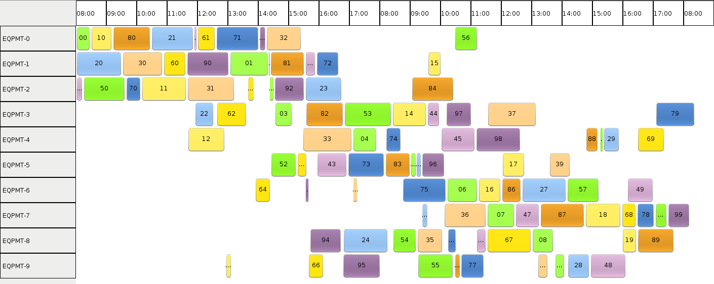
Literature mentions the minimum makespan for FT10 is 930 time units. With this implementation, I could find a „reasonably good“ solution in about two seconds:

23:08:05.091 [l-2-thread-1] INFO Solving started: time spent (21), best score (-100init/0hard/-24480soft), environment mode (REPRODUCIBLE), random (JDK with seed 0).
23:08:05.272 [l-2-thread-1] DEBUG CH step (0), time spent (202), score (-99init/0hard/-24480soft), selected move count (1700), picked move (00 {null -> StartTime{time=0}}).
[...]
23:08:07.267 [l-2-thread-1] DEBUG LS step (0), time spent (2197), score (0hard/-12651721soft), best score (0hard/-12651721soft), accepted/selected move count (1/278), picked move (80 {StartTime{time=72} -> StartTime{time=809}}).

The makespan I could achieve slightly varies based on solver configurations, but – strangely – also based on the sequence of the entities in the solver input. Some best schedules were in the range of makespan 1100. While, by manually validating those schedules, they seem to have little improvement potential, they are still ~18 percent off the optimum.

I am just in the middle of a learning curve with Optaplanner, so I assume there is more tweaking or model changes that would further improve the schedule.

A commercial solver could come up with the optimum in ~6 seconds. Let’s see if Optaplanner can be fine-tuned to go further to the optimum… it has still four more seconds to go 🙂